The 1836 Tithe Commutation Commission files contain a huge amount of highly useful data, including the pastoral rents and yields of some parishes in the south-west of England. I want to see how the rent changed with distance from the main market, which was London. No trucks or railways then, so the animals had to be driven overland. This was expensive no least because the animals was sold by weight and a long journey caused significant weight loss. The regression equation works fine. I used elevation as an independent variable, and the full equation was: Pasture Rent = elevation + Pasture Yield + London Distance. As expected, elevation and London Distance had negative signs. A map of the parishes colored with their rent is below. Only three categories shown. The darker the blue the higher the rent. The escarpments that existed at that time are also shown.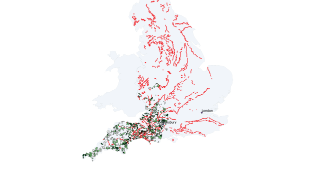
. Notice how the higher rents are all closer to London. But how about the non-linear effects of elevation and distance? If the farm was very high up then the animals would have to go up hill and down dale? I used the mgcv package in R for this. Here is a contour plot showing the rents:
pasturecontour
Look at the contour lines where you can see the rents. They are curved especially about halfway along. This reflects the topography of Devon.


